The filled-in Julia set
K
(
f
)
{\displaystyle K(f)}


Formal definition
The filled-in Julia set
K
(
f
)
{\displaystyle K(f)}


-
C
{\displaystyle \mathbb {C} }
is the set of complex numbers
-
f
(
k
)
(
z
)
{\displaystyle f^{(k)}(z)}
is the k {\displaystyle k}
-fold composition of f {\displaystyle f}
Relation to the Fatou set
The filled-in Julia set is the (absolute) complement of the attractive basin of infinity.
K
(
f
)
=
C
∖
A
f
(
∞
)
{\displaystyle K(f)=\mathbb {C} \setminus A_{f}(\infty )}

The attractive basin of infinity is one of the components of the Fatou set.
A
f
(
∞
)
=
F
∞
{\displaystyle A_{f}(\infty )=F_{\infty }}

In other words, the filled-in Julia set is the complement of the unbounded Fatou component:
K
(
f
)
=
F
∞
C
.
{\displaystyle K(f)=F_{\infty }^{C}.}

Relation between Julia, filled-in Julia set and attractive basin of infinity
The Julia set is the common boundary of the filled-in Julia set and the attractive basin of infinity
J
(
f
)
=
∂
K
(
f
)
=
∂
A
f
(
∞
)
{\displaystyle J(f)=\partial K(f)=\partial A_{f}(\infty )}


A
f
(
∞
)
=
d
e
f
{
z
∈
C
:
f
(
k
)
(
z
)
→
∞
a
s
k
→
∞
}
.
{\displaystyle A_{f}(\infty )\ {\overset {\underset {\mathrm {def} }{}}{=}}\ \{z\in \mathbb {C} :f^{(k)}(z)\to \infty \ as\ k\to \infty \}.}

If the filled-in Julia set has no interior then the Julia set coincides with the filled-in Julia set. This happens when all the critical points of
f
{\displaystyle f}
Spine
 Rabbit Julia set with spine
 Basilica Julia set with spine


The most studied polynomials are probably those of the form
f
(
z
)
=
z
2
+
c
{\displaystyle f(z)=z^{2}+c}


![{\displaystyle S_{c}=\left[-\beta ,\beta \right]}](https://wikimedia.org/api/rest_v1/media/math/render/svg/0dc28d767679ab7c75c23b245f5213dc2e38cb52)
- spine lies inside
K
{\displaystyle K}
- spine is invariant under 180 degree rotation,
- spine is a finite topological tree,
- Critical point
z
c
r
=
0
{\displaystyle z_{cr}=0}
always belongs to the spine.[3]
-
β
{\displaystyle \beta }
,
-
−
β
{\displaystyle -\beta }
.
Algorithms for constructing the spine:
- detailed version is described by A. Douady[4]
- Simplified version of algorithm:
- connect
−
β
{\displaystyle -\beta }
- when
K
{\displaystyle K}
- otherwise take the shortest way that contains
0
{\displaystyle 0}
.[5]
- connect
−
β
{\displaystyle -\beta }
Curve
R
{\displaystyle R}


Images
 Filled Julia set for fc, c=1−φ=−0.618033988749…, where φ is the Golden ratio
 Filled Julia with no interior = Julia set. This example has c=i.
 Filled Julia set for c=−1+0.1*i. Here Julia set is the boundary of filled-in Julia set.
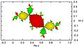
 Filled Julia set for c = −0.8 + 0.156i.
 Filled Julia set for c = 0.285 + 0.01i.
 Filled Julia set for c = −1.476.


Names
- airplane[6]
- Douady rabbit
- dragon
- basilica or San Marco fractal or San Marco dragon
- cauliflower
- dendrite
- Siegel disc
Notes
- Douglas C. Ravenel: External angles in the Mandelbrot set: the work of Douady and Hubbard. University of Rochester Archived 2012-02-08 at the Wayback Machine
- John Milnor : Pasting Together Julia Sets: A Worked Out Example of Mating. Experimental Mathematics Volume 13 (2004)
- Saaed Zakeri: Biaccessiblility in quadratic Julia sets I: The locally-connected case
- A. Douady, “Algorithms for computing angles in the Mandelbrot set,” in Chaotic Dynamics and Fractals, M. Barnsley and S. G. Demko, Eds., vol. 2 of Notes and Reports in Mathematics in Science and Engineering, pp. 155–168, Academic Press, Atlanta, Georgia, USA, 1986.
- K M. Brucks, H Bruin : Topics from One-Dimensional Dynamics Series: London Mathematical Society Student Texts (No. 62) page 257
- The Mandelbrot Set And Its Associated Julia Sets by Hermann Karcher
References
- Peitgen Heinz-Otto, Richter, P.H. : The beauty of fractals: Images of Complex Dynamical Systems. Springer-Verlag 1986. ISBN 978-0-387-15851-8.
- Bodil Branner : Holomorphic dynamical systems in the complex plane. Department of Mathematics Technical University of Denmark, MAT-Report no. 1996-42.