In physics, the Maxwell–Jüttner distribution, sometimes called Jüttner–Synge distribution, is the distribution of speeds of particles in a hypothetical gas of relativistic particles. Similar to the Maxwell–Boltzmann distribution, the Maxwell–Jüttner distribution considers a classical ideal gas where the particles are dilute and do not significantly interact with each other. The distinction from Maxwell–Boltzmann's case is that effects of special relativity are taken into account. In the limit of low temperatures
T
{\displaystyle T}


The distribution can be attributed to Ferencz Jüttner, who derived it in 1911.[1] It has become known as the Maxwell–Jüttner distribution by analogy to the name Maxwell–Boltzmann distribution that is commonly used to refer to Maxwell's or Maxwellian distribution.
Definition
_for_electron_gas_at_different_temperatures.svg)
As the gas becomes hotter and
k
B
T
{\displaystyle k_{\text{B}}T}



f
(
γ
)
d
γ
=
γ
2
β
(
γ
)
θ
K
2
(
1
θ
)
e
−
γ
/
θ
d
γ
{\displaystyle f(\gamma )\,\mathrm {d} \gamma ={\frac {\gamma ^{2}\,\beta (\gamma )}{\theta \operatorname {K} _{2}\!\left({\frac {1}{\theta }}\right)}}e^{-{\gamma }/{\theta }}\,\mathrm {d} \gamma }

where
β
=
v
c
=
1
−
1
/
γ
2
{\textstyle \beta ={\frac {v}{c}}={\sqrt {1-1/\gamma ^{2}}}}


Alternatively, this can be written in terms of the momentum as
f
(
p
)
d
3
p
=
1
4
π
θ
K
2
(
1
θ
)
e
−
γ
(
p
)
/
θ
d
3
p
(
m
c
)
3
{\displaystyle f(\mathbf {p} )\,\mathrm {d} ^{3}\mathbf {p} ={\frac {1}{4\pi \theta \operatorname {K} _{2}\!\left({\frac {1}{\theta }}\right)}}e^{-\gamma (p)/\theta }\,{\frac {\mathrm {d} ^{3}\mathbf {p} }{(mc)^{3}}}}

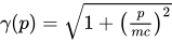

The Maxwell–Jüttner equation is covariant, but not manifestly so, and the temperature of the gas does not vary with the gross speed of the gas.[3]
Jüttner distribution graph
A visual representation of the distribution in particle velocities for plasmas at four different temperatures:[4]
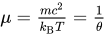
Where thermal parameter has been defined as
μ
=
m
c
2
k
B
T
=
1
θ
{\textstyle \mu ={\frac {mc^{2}}{k_{\text{B}}T}}={\frac {1}{\theta }}}
The four general limits are:
- ultrarelativistic temperatures
μ
≪
1
⟺
θ
≫
1
{\displaystyle \mu \ll 1\iff \theta \gg 1}
( k B T ≫ m c 2 {\displaystyle k_{\text{B}}T\gg mc^{2}}
),
- relativistic temperatures:
μ
<
1
⟺
θ
>
1
{\displaystyle \mu <1\iff \theta >1}
( k B T > m c 2 {\displaystyle k_{\text{B}}T>mc^{2}}
),
- weakly (or mildly) relativistic temperatures:
μ
>
1
⟺
θ
<
1
{\displaystyle \mu >1\iff \theta <1}
( k B T < m c 2 {\displaystyle k_{\text{B}}T<mc^{2}}
),
- low temperatures:
μ
≫
1
⟺
θ
≪
1
{\displaystyle \mu \gg 1\iff \theta \ll 1}
( k B T ≪ m c 2 {\displaystyle k_{\text{B}}T\ll mc^{2}}
),
Limitations
Some limitations of the Maxwell–Jüttner distributions are shared with the classical ideal gas: neglect of interactions, and neglect of quantum effects. An additional limitation (not important in the classical ideal gas) is that the Maxwell–Jüttner distribution neglects antiparticles.
If particle-antiparticle creation is allowed, then once the thermal energy
k
B
T
{\displaystyle k_{\text{B}}T}
Perhaps most significantly, the basic MB distribution has two main issues: it does not extend to particles moving at relativistic speeds, and it assumes anisotropic temperature (where each DoF does not have the same translational kinetic energy). While the classic Maxwell–Jüttner distribution generalizes for the case of special relativity, it fails to consider the anisotropic description.
Derivation
The Maxwell–Boltzmann (MB) distribution
f
MB
{\displaystyle f_{\text{MB}}}


f
MB
(
p
;
v
th
)
d
n
p
=
(
π
m
2
v
th
2
)
−
n
/
2
e
−
p
2
/
2
m
k
B
T
d
n
p
,
v
th
≡
2
k
B
T
/
m
,
f
MB
(
ε
;
T
)
d
ε
=
(
k
B
T
)
−
n
/
2
Γ
(
n
/
2
)
e
−
ε
/
k
B
T
ε
1
2
n
−
1
d
ε
{\displaystyle {\begin{aligned}f_{\text{MB}}(\mathbf {p} ;v_{\text{th}})\,\mathrm {d} ^{n}\mathbf {p} &=\left(\pi m^{2}v_{\text{th}}^{2}\right)^{-n/2}e^{-{\frac {\mathbf {p} ^{2}/2m}{k_{\text{B}}T}}}\,\mathrm {d} ^{n}\mathbf {p} ,&v_{\text{th}}\equiv {\sqrt {2{k_{\text{B}}T}/{m}}},\\[1ex]f_{\text{MB}}(\varepsilon ;T)\,\mathrm {d} \varepsilon &={\frac {\left(k_{\text{B}}T\right)^{-n/2}}{\Gamma {\left(n/2\right)}}}e^{-\varepsilon /{k_{\text{B}}T}}\varepsilon ^{{\frac {1}{2}}n-1}\,\mathrm {d} \varepsilon \end{aligned}}}
![{\displaystyle {\begin{aligned}f_{\text{MB}}(\mathbf {p} ;v_{\text{th}})\,\mathrm {d} ^{n}\mathbf {p} &=\left(\pi m^{2}v_{\text{th}}^{2}\right)^{-n/2}e^{-{\frac {\mathbf {p} ^{2}/2m}{k_{\text{B}}T}}}\,\mathrm {d} ^{n}\mathbf {p} ,&v_{\text{th}}\equiv {\sqrt {2{k_{\text{B}}T}/{m}}},\\[1ex]f_{\text{MB}}(\varepsilon ;T)\,\mathrm {d} \varepsilon &={\frac {\left(k_{\text{B}}T\right)^{-n/2}}{\Gamma {\left(n/2\right)}}}e^{-\varepsilon /{k_{\text{B}}T}}\varepsilon ^{{\frac {1}{2}}n-1}\,\mathrm {d} \varepsilon \end{aligned}}}](https://wikimedia.org/api/rest_v1/media/math/render/svg/e12145c78a9a90f330319c4ec50d73c9c2defe8a) | 1 |
where the low-energy limit (non-relativistic) can be expressed as
u
≪
c
{\textstyle u\ll c}


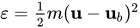
The relativistic generalization of Eq. (1), that is, the Maxwell–Jüttner (MJ) distribution, is given by:
f
MJ
(
γ
)
∝
γ
2
β
(
γ
)
e
−
γ
/
θ
,
{\displaystyle f_{\text{MJ}}(\gamma )\propto \gamma ^{2}\beta (\gamma )\,e^{-\gamma /\theta },}
 | 2 |
where
θ
≡
k
B
T
/
m
c
2
{\textstyle \theta \equiv {k_{\text{B}}T}/{mc^{2}}}


p
=
m
c
γ
(
β
)
β
,
E
(
β
)
=
γ
(
β
)
m
c
2
.
{\displaystyle {\begin{aligned}\mathbf {p} &=mc\,\gamma {\left(\beta \right)}\,\mathbf {\beta } ,&E{\left(\beta \right)}&=\gamma (\beta )\,mc^{2}.\end{aligned}}}

While the kinetic energy is given by
ε
=
E
−
m
c
2
=
(
γ
−
1
)
m
c
2
{\displaystyle \varepsilon =E-mc^{2}=(\gamma -1)\,mc^{2}}


f
MJ
(
E
)
∝
e
−
E
k
B
T
∝
e
−
γ
/
θ
{\displaystyle f_{\text{MJ}}\left(E\right)\propto e^{-{\frac {E}{k_{\text{B}}T}}}\propto e^{-\gamma /\theta }}

(Note that
E
{\displaystyle E}


f
MJ
(
γ
)
∝
p
(
γ
)
n
−
1
d
p
(
γ
)
d
γ
e
−
γ
/
θ
{\displaystyle f_{\text{MJ}}(\gamma )\propto p(\gamma )^{n-1}{\frac {\mathrm {d} p(\gamma )}{\mathrm {d} \gamma }}\,e^{-\gamma /\theta }}

So that:
∫
f
MJ
(
p
)
d
p
1
⋯
d
p
n
∝
∫
e
−
E
(
p
)
k
B
T
d
p
1
⋯
d
p
n
=
∫
e
−
E
(
γ
Ω
n
)
k
B
T
d
Ω
n
p
n
−
1
d
p
=
∫
Ω
n
e
−
E
(
γ
Ω
n
)
k
B
T
(
p
(
γ
)
n
−
1
d
p
(
γ
)
d
γ
)
d
Ω
n
d
γ
{\displaystyle {\begin{aligned}\int f_{\text{MJ}}(\mathbf {p} )\,\mathrm {d} p_{1}\cdots \mathrm {d} p_{n}&\propto \int e^{-{\frac {E(\mathbf {p} )}{k_{\text{B}}T}}}\,\mathrm {d} p_{1}\cdots \mathrm {d} p_{n}\\[1ex]&=\int e^{-{\frac {E(\gamma \Omega _{n})}{k_{\text{B}}T}}}\,\mathrm {d} \Omega _{n}\,p^{n-1}\,\mathrm {d} p\\[1ex]&=\int _{\Omega _{n}}e^{-{\frac {E(\gamma \Omega _{n})}{k_{\text{B}}T}}}\,\left(p(\gamma )^{n-1}{\frac {\mathrm {d} p(\gamma )}{\mathrm {d} \gamma }}\right)\mathrm {d} \Omega _{n}\,\mathrm {d} \gamma \end{aligned}}}
![{\displaystyle {\begin{aligned}\int f_{\text{MJ}}(\mathbf {p} )\,\mathrm {d} p_{1}\cdots \mathrm {d} p_{n}&\propto \int e^{-{\frac {E(\mathbf {p} )}{k_{\text{B}}T}}}\,\mathrm {d} p_{1}\cdots \mathrm {d} p_{n}\\[1ex]&=\int e^{-{\frac {E(\gamma \Omega _{n})}{k_{\text{B}}T}}}\,\mathrm {d} \Omega _{n}\,p^{n-1}\,\mathrm {d} p\\[1ex]&=\int _{\Omega _{n}}e^{-{\frac {E(\gamma \Omega _{n})}{k_{\text{B}}T}}}\,\left(p(\gamma )^{n-1}{\frac {\mathrm {d} p(\gamma )}{\mathrm {d} \gamma }}\right)\mathrm {d} \Omega _{n}\,\mathrm {d} \gamma \end{aligned}}}](https://wikimedia.org/api/rest_v1/media/math/render/svg/82258893125a1d79598d0aee1c9f2ee5bba54bd3)
Where
d
Ω
n
{\displaystyle \mathrm {d} \Omega _{n}}

∫
f
MJ
(
p
)
d
p
1
⋯
d
p
n
∝
∫
e
−
E
(
p
)
k
B
T
(
p
(
γ
)
n
−
1
d
p
(
γ
)
d
γ
)
d
Ω
n
d
γ
≡
∫
Ω
n
d
Ω
n
∫
f
MJ
(
γ
)
d
γ
{\displaystyle \int f_{\text{MJ}}(p)\,\mathrm {d} p_{1}\cdots \mathrm {d} p_{n}\propto \int e^{-{\frac {E(p)}{k_{\text{B}}T}}}\left(p(\gamma )^{n-1}{\frac {\mathrm {d} p(\gamma )}{\mathrm {d} \gamma }}\right)\mathrm {d} \Omega _{n}\,\mathrm {d} \gamma \equiv \int _{\Omega _{n}}\mathrm {d} \Omega _{n}\,\int f_{\text{MJ}}(\gamma )\,\mathrm {d} \gamma }

or
f
MJ
(
γ
)
∝
e
−
E
(
γ
)
k
B
T
p
(
γ
)
n
−
1
d
p
(
γ
)
d
γ
{\displaystyle f_{\text{MJ}}(\gamma )\propto e^{-{\frac {E(\gamma )}{k_{\text{B}}T}}}\,p(\gamma )^{n-1}{\frac {\mathrm {d} p(\gamma )}{\mathrm {d} \gamma }}}

Then,
d
(
γ
β
)
=
γ
(
γ
2
−
1
)
−
1
2
d
γ
=
β
−
1
d
γ
{\displaystyle \mathrm {d} (\gamma \beta )=\gamma \left(\gamma ^{2}-1\right)^{-{\frac {1}{2}}}\mathrm {d} \gamma =\beta ^{-1}\,\mathrm {d} \gamma }

p
(
γ
)
n
−
1
d
p
(
γ
)
d
γ
=
(
m
c
)
n
(
γ
β
)
n
−
1
d
(
γ
β
)
d
γ
=
(
m
c
)
n
γ
n
−
1
β
n
−
2
,
{\displaystyle {\begin{aligned}p\left(\gamma \right)^{n-1}{\frac {\mathrm {d} p\left(\gamma \right)}{\mathrm {d} \gamma }}&=\left(mc\right)^{n}\left(\gamma \beta \right)^{n-1}{\frac {\mathrm {d} (\gamma \beta )}{\mathrm {d} \gamma }}\\&=\left(mc\right)^{n}\gamma ^{n-1}\beta ^{n-2},\end{aligned}}}

Or:
f
MJ
(
γ
)
∝
γ
n
−
1
β
n
−
2
e
−
γ
θ
∝
γ
(
γ
2
−
1
)
n
2
−
1
e
−
γ
θ
{\displaystyle f_{\text{MJ}}(\gamma )\propto \gamma ^{n-1}\beta ^{n-2}e^{-{\frac {\gamma }{\theta }}}\propto \gamma \left(\gamma ^{2}-1\right)^{{\frac {n}{2}}-1}\,e^{-{\frac {\gamma }{\theta }}}}
 | 3 |
Now, because
E
k
B
T
=
γ
θ
{\displaystyle {\frac {E}{k_{\text{B}}T}}={\frac {\gamma }{\theta }}}


And the angular integration:
d
p
1
⋯
d
p
n
=
B
n
p
n
−
1
d
p
=
1
2
B
n
(
m
c
)
n
(
(
p
m
c
)
2
)
n
2
−
1
d
(
p
m
c
)
2
,
{\displaystyle \mathrm {d} p_{1}\cdots \mathrm {d} p_{n}=B_{n}p^{n-1}\,\mathrm {d} p={\frac {1}{2}}B_{n}\left(mc\right)^{n}\left(\left({\frac {p}{mc}}\right)^{2}\right)^{{\frac {n}{2}}-1}\,\mathrm {d} {\left({\frac {p}{mc}}\right)^{2}},}

Where
B
n
=
2
π
n
/
2
Γ
(
n
/
2
)
{\displaystyle B_{n}={\frac {2\pi ^{n/2}}{\Gamma {\left(n/2\right)}}}}


![{\displaystyle {\begin{aligned}1&=\int _{-\infty }^{\infty }f_{\text{MJ}}(\mathbf {p} ;\theta )\,\mathrm {d} p_{1}\cdots \mathrm {d} p_{n}\\[1ex]&={\frac {N}{2}}B_{n}\left(mc\right)^{n}\,\int _{1}^{\infty }e^{-{\frac {\gamma }{\theta }}}\left(\gamma ^{2}-1\right)^{{\frac {n}{2}}-1}\mathrm {d} (\gamma ^{2}-1)\\[1ex]&={\frac {N}{2}}B_{n}\left({\frac {n}{2}}\right)^{-1}\left(mc\right)^{n}\theta ^{-1}\,\int _{1}^{\infty }e^{\frac {\gamma }{\theta }}\left(\gamma ^{2}-1\right)^{\frac {n}{2}}\mathrm {d} \gamma \\[1ex]&={\frac {N}{2}}B_{n}\left({\frac {n}{2}}\right)^{-1}\left(mc\right)^{n}\theta ^{-1}\,I_{n},\end{aligned}}}](https://wikimedia.org/api/rest_v1/media/math/render/svg/82df0ebf0e8fb9dbd501e1c6f44ef624f3972c3b)
Where one has defined the integral:
I
n
≡
∫
1
∞
e
−
γ
/
θ
(
γ
2
−
1
)
n
/
2
d
γ
.
{\displaystyle I_{n}\equiv \int _{1}^{\infty }e^{-\gamma /\theta }\left(\gamma ^{2}-1\right)^{n/2}\mathrm {d} \gamma .}

The Macdonald function (Modified Bessel function of the second kind) (Abramowitz and Stegun, 1972, p.376) is defined by:
K
ν
(
z
)
≡
π
1
2
(
1
2
z
)
ν
Γ
(
ν
+
1
2
)
∫
1
∞
e
−
z
γ
(
γ
2
−
1
)
ν
−
1
2
d
γ
{\displaystyle \operatorname {K} _{\nu }(z)\equiv {\frac {\pi ^{\frac {1}{2}}\left({\frac {1}{2}}z\right)^{\nu }}{\Gamma {\left(\nu +{\frac {1}{2}}\right)}}}\int _{1}^{\infty }e^{-z\gamma }\left(\gamma ^{2}-1\right)^{\nu -{\frac {1}{2}}}\,\mathrm {d} \gamma }

So that, by setting
ν
=
n
+
1
2
,
z
=
1
θ
{\displaystyle \nu ={\frac {n+1}{2}},\ z={\frac {1}{\theta }}}

I
n
=
Γ
(
n
2
+
1
)
π
−
1
2
K
n
+
1
2
(
1
θ
)
(
2
θ
)
n
+
1
2
{\displaystyle I_{n}=\Gamma {\left({\frac {n}{2}}+1\right)}\pi ^{-{\frac {1}{2}}}\operatorname {K} _{\frac {n+1}{2}}{\!\!\left({\frac {1}{\theta }}\right)}\left(2\theta \right)^{\frac {n+1}{2}}}

Hence,
N
−
1
=
π
n
2
Γ
(
n
2
)
(
n
2
)
−
1
Γ
(
n
2
+
1
)
π
−
1
2
K
n
+
1
2
(
1
θ
)
(
m
c
)
n
(
2
θ
)
n
+
1
2
=
π
n
−
1
2
2
−
n
+
1
2
(
m
c
)
n
θ
n
−
1
2
K
n
+
1
2
(
1
θ
)
,
{\displaystyle {\begin{aligned}N^{-1}&={\frac {\pi ^{\frac {n}{2}}}{\Gamma {\left({\frac {n}{2}}\right)}}}\left({\frac {n}{2}}\right)^{-1}\Gamma {\left({\frac {n}{2}}+1\right)}\pi ^{-{\frac {1}{2}}}\operatorname {K} _{\frac {n+1}{2}}{\!\!\left({\frac {1}{\theta }}\right)}\,\left(mc\right)^{n}\left(2\theta \right)^{\frac {n+1}{2}}\\[1ex]&=\pi ^{\frac {n-1}{2}}2^{-{\frac {n+1}{2}}}\left(mc\right)^{n}\,\theta ^{\frac {n-1}{2}}\operatorname {K} _{\frac {n+1}{2}}{\!\!\left({\frac {1}{\theta }}\right)},\end{aligned}}}
![{\displaystyle {\begin{aligned}N^{-1}&={\frac {\pi ^{\frac {n}{2}}}{\Gamma {\left({\frac {n}{2}}\right)}}}\left({\frac {n}{2}}\right)^{-1}\Gamma {\left({\frac {n}{2}}+1\right)}\pi ^{-{\frac {1}{2}}}\operatorname {K} _{\frac {n+1}{2}}{\!\!\left({\frac {1}{\theta }}\right)}\,\left(mc\right)^{n}\left(2\theta \right)^{\frac {n+1}{2}}\\[1ex]&=\pi ^{\frac {n-1}{2}}2^{-{\frac {n+1}{2}}}\left(mc\right)^{n}\,\theta ^{\frac {n-1}{2}}\operatorname {K} _{\frac {n+1}{2}}{\!\!\left({\frac {1}{\theta }}\right)},\end{aligned}}}](https://wikimedia.org/api/rest_v1/media/math/render/svg/35f48bd705ed007e956890a0c8fa90b77fc4a728)
Or
N
=
π
1
−
n
2
2
−
n
+
1
2
(
m
c
)
−
n
θ
1
−
n
2
K
n
+
1
2
(
1
θ
)
−
1
,
{\displaystyle N=\pi ^{\frac {1-n}{2}}2^{-{\frac {n+1}{2}}}\left(mc\right)^{-n}\,\theta ^{\frac {1-n}{2}}\operatorname {K} _{\frac {n+1}{2}}{\!\!\left({\frac {1}{\theta }}\right)}^{-1},}

The inverse of the normalization constant gives the partition function
Z
≡
1
N
{\displaystyle Z\equiv {\frac {1}{N}}}

Z
=
π
n
−
1
2
2
−
n
+
1
2
(
m
c
)
n
θ
n
−
1
2
K
n
+
1
2
(
1
θ
)
,
{\displaystyle Z=\pi ^{\frac {n-1}{2}}2^{-{\frac {n+1}{2}}}\left(mc\right)^{n}\,\theta ^{\frac {n-1}{2}}\operatorname {K} _{\frac {n+1}{2}}{\!\!\left({\frac {1}{\theta }}\right)},}

Therefore, the normalized distribution is:
f
MJ
(
p
;
θ
)
d
p
1
⋯
d
p
n
=
π
1
−
n
2
2
−
n
+
1
2
(
m
c
)
−
n
θ
1
−
n
2
e
−
γ
(
p
)
/
θ
K
n
+
1
2
(
1
θ
)
d
p
1
⋯
d
p
n
{\displaystyle f_{\text{MJ}}(p;\theta )\,\mathrm {d} p_{1}\cdots \mathrm {d} p_{n}=\pi ^{\frac {1-n}{2}}2^{-{\frac {n+1}{2}}}(mc)^{-n}\,\theta ^{\frac {1-n}{2}}{\frac {e^{-\gamma (p)/\theta }}{\operatorname {K} _{\frac {n+1}{2}}{\!\!\left({\frac {1}{\theta }}\right)}}}\,\mathrm {d} p_{1}\cdots \mathrm {d} p_{n}}

Or one may derive the normalised distribution in terms of:
f
MJ
(
γ
;
θ
)
d
γ
=
π
1
2
2
1
−
n
2
Γ
(
n
2
)
θ
1
−
n
2
e
−
γ
/
θ
K
n
+
1
2
(
1
θ
)
(
γ
2
−
1
)
n
2
−
1
γ
d
γ
{\displaystyle f_{\text{MJ}}(\gamma ;\theta )\,\mathrm {d} \gamma ={\frac {\pi ^{\frac {1}{2}}2^{\frac {1-n}{2}}}{\Gamma {\left({\frac {n}{2}}\right)}}}\theta ^{\frac {1-n}{2}}{\frac {e^{-\gamma /\theta }}{\operatorname {K} _{\frac {n+1}{2}}{\!\!\left({\frac {1}{\theta }}\right)}}}\left(\gamma ^{2}-1\right)^{{\frac {n}{2}}-1}\gamma \,\mathrm {d} \gamma }

Note that
θ
{\displaystyle \theta }
Also useful is the expression of the distribution in the velocity space.[7] Given that
d
(
β
γ
)
d
β
=
γ
3
{\displaystyle {\frac {\mathrm {d} (\beta \gamma )}{\mathrm {d} \beta }}=\gamma ^{3}}

d
p
1
⋯
d
p
n
=
p
n
−
1
d
p
d
Ω
n
=
(
m
c
)
n
γ
n
−
1
β
n
−
1
d
(
β
γ
)
d
β
d
β
d
Ω
n
=
(
m
c
)
n
γ
n
+
2
β
n
−
1
d
β
d
Ω
n
=
(
m
c
)
n
γ
n
+
2
d
β
1
⋯
d
β
n
{\displaystyle {\begin{aligned}\mathrm {d} p_{1}\cdots \mathrm {d} p_{n}=p^{n-1}\,\mathrm {d} p\,\mathrm {d} \Omega _{n}&=\left(mc\right)^{n}\gamma ^{n-1}\beta ^{n-1}{\frac {\mathrm {d} (\beta \gamma )}{\mathrm {d} \beta }}\,\mathrm {d} \beta \,\mathrm {d} \Omega _{n}\\[1ex]&=\left(mc\right)^{n}\gamma ^{n+2}\beta ^{n-1}\,\mathrm {d} \beta \,\mathrm {d} \Omega _{n}\\[1ex]&=\left(mc\right)^{n}\gamma ^{n+2}\,\mathrm {d} \beta _{1}\cdots \mathrm {d} \beta _{n}\end{aligned}}}
![{\displaystyle {\begin{aligned}\mathrm {d} p_{1}\cdots \mathrm {d} p_{n}=p^{n-1}\,\mathrm {d} p\,\mathrm {d} \Omega _{n}&=\left(mc\right)^{n}\gamma ^{n-1}\beta ^{n-1}{\frac {\mathrm {d} (\beta \gamma )}{\mathrm {d} \beta }}\,\mathrm {d} \beta \,\mathrm {d} \Omega _{n}\\[1ex]&=\left(mc\right)^{n}\gamma ^{n+2}\beta ^{n-1}\,\mathrm {d} \beta \,\mathrm {d} \Omega _{n}\\[1ex]&=\left(mc\right)^{n}\gamma ^{n+2}\,\mathrm {d} \beta _{1}\cdots \mathrm {d} \beta _{n}\end{aligned}}}](https://wikimedia.org/api/rest_v1/media/math/render/svg/0ba4b1b26df512419a4e96f6ccf7f3b8d75bacca)
Hence
f
MJ
(
β
;
θ
)
d
β
1
⋯
d
β
n
=
π
1
−
n
2
2
−
n
+
1
2
θ
1
−
n
2
e
−
γ
(
β
)
/
θ
K
n
+
1
2
(
1
θ
)
γ
(
β
)
n
+
2
d
β
1
⋯
d
β
n
{\displaystyle f_{\text{MJ}}(\mathbf {\beta } ;\theta )\,\mathrm {d} \beta _{1}\cdots \mathrm {d} \beta _{n}=\pi ^{\frac {1-n}{2}}2^{-{\frac {n+1}{2}}}\,\theta ^{\frac {1-n}{2}}{\frac {e^{-\gamma (\beta )/\theta }}{\operatorname {K} _{\frac {n+1}{2}}{\!\!\left({\frac {1}{\theta }}\right)}}}\,\gamma (\beta )^{n+2}\,\mathrm {d} \beta _{1}\cdots \mathrm {d} \beta _{n}}

Take
n
=
3
{\displaystyle n=3}

f
MJ
(
p
;
θ
)
d
p
1
d
p
2
d
p
3
=
e
−
γ
(
p
)
/
θ
θ
K
2
(
1
/
θ
)
d
p
1
d
p
2
d
p
3
4
π
(
m
c
)
3
,
f
MJ
(
γ
;
θ
)
d
γ
=
e
−
γ
/
θ
(
γ
2
−
1
)
1
/
2
θ
K
2
(
1
/
θ
)
γ
d
γ
,
f
MJ
(
β
;
θ
)
d
β
1
d
β
2
d
β
3
=
e
−
γ
(
β
)
/
θ
γ
(
β
)
5
θ
K
2
(
1
/
θ
)
d
β
1
d
β
2
d
β
3
4
π
.
{\displaystyle {\begin{aligned}f_{\text{MJ}}(p;\theta )\,\mathrm {d} p_{1}\,\mathrm {d} p_{2}\,\mathrm {d} p_{3}&={\frac {e^{-{\gamma (\mathbf {p} )/\theta }}}{\theta \,\operatorname {K} _{2}{\!\left(1/\theta \right)}}}\,{\frac {\mathrm {d} p_{1}\,\mathrm {d} p_{2}\,\mathrm {d} p_{3}}{4\pi \left(mc\right)^{3}}},\\[1ex]f_{\text{MJ}}(\gamma ;\theta )\,\mathrm {d} \gamma &={\frac {e^{-\gamma /\theta }\left(\gamma ^{2}-1\right)^{1/2}}{\theta \,\operatorname {K} _{2}{\!\left(1/\theta \right)}}}\,\gamma \,\mathrm {d} \gamma ,\\[1ex]f_{\text{MJ}}(\beta ;\theta )\,\mathrm {d} \beta _{1}\,\mathrm {d} \beta _{2}\,\mathrm {d} \beta _{3}&={\frac {e^{-\gamma (\beta )/\theta }\gamma (\beta )^{5}}{\theta \operatorname {K} _{2}{\!\left(1/\theta \right)}}}\,{\frac {\mathrm {d} \beta _{1}\,\mathrm {d} \beta _{2}\,\mathrm {d} \beta _{3}}{4\pi }}.\end{aligned}}}
![{\displaystyle {\begin{aligned}f_{\text{MJ}}(p;\theta )\,\mathrm {d} p_{1}\,\mathrm {d} p_{2}\,\mathrm {d} p_{3}&={\frac {e^{-{\gamma (\mathbf {p} )/\theta }}}{\theta \,\operatorname {K} _{2}{\!\left(1/\theta \right)}}}\,{\frac {\mathrm {d} p_{1}\,\mathrm {d} p_{2}\,\mathrm {d} p_{3}}{4\pi \left(mc\right)^{3}}},\\[1ex]f_{\text{MJ}}(\gamma ;\theta )\,\mathrm {d} \gamma &={\frac {e^{-\gamma /\theta }\left(\gamma ^{2}-1\right)^{1/2}}{\theta \,\operatorname {K} _{2}{\!\left(1/\theta \right)}}}\,\gamma \,\mathrm {d} \gamma ,\\[1ex]f_{\text{MJ}}(\beta ;\theta )\,\mathrm {d} \beta _{1}\,\mathrm {d} \beta _{2}\,\mathrm {d} \beta _{3}&={\frac {e^{-\gamma (\beta )/\theta }\gamma (\beta )^{5}}{\theta \operatorname {K} _{2}{\!\left(1/\theta \right)}}}\,{\frac {\mathrm {d} \beta _{1}\,\mathrm {d} \beta _{2}\,\mathrm {d} \beta _{3}}{4\pi }}.\end{aligned}}}](https://wikimedia.org/api/rest_v1/media/math/render/svg/6fcd4fea6ca243390591e804e26e2f6934ec77b3)
Note that when the MB distribution clearly deviates from the MJ distribution of the same temperature and dimensionality, one can misinterpret and deduce a different MB distribution that will give a good approximation to the MJ distribution. This new MB distribution can be either:
- a convected MB distribution, that is, an MB distribution with the same dimensionality, but with different temperature
T
MB
{\displaystyle T_{\text{MB}}}
and bulk speed u b {\displaystyle \mathbf {u} _{b}}
)
- an MB distribution with the same bulk speed, but with different temperature
T
MB
{\displaystyle T_{\text{MB}}}
. These two types of approximations are illustrated.
Other properties
The MJ probability density function is given by:
f
MJ
(
γ
)
d
γ
=
γ
2
β
(
γ
)
θ
K
2
(
1
/
θ
)
e
−
γ
/
θ
d
γ
{\displaystyle f_{\text{MJ}}(\gamma )\,\mathrm {d} \gamma ={\frac {\gamma ^{2}\,\beta (\gamma )}{\theta \operatorname {K} _{2}{\!\left(1/\theta \right)}}}\,e^{-{\gamma }/{\theta }}\,\mathrm {d} \gamma }

This means that a relativistic non-quantum particle with parameter
θ
{\displaystyle \theta }

![{\displaystyle [\gamma ,\gamma +\mathrm {d} \gamma ]}](https://wikimedia.org/api/rest_v1/media/math/render/svg/4092e8fc346d7fe84225dc6a1af2e47be6e15487)
Cumulative distribution function
The MJ cumulative distribution function is given by:
F
MJ
(
γ
)
=
1
θ
K
2
(
1
/
θ
)
∫
1
γ
γ
′
2
1
−
1
γ
′
2
e
−
γ
′
/
θ
d
γ
′
{\displaystyle F_{\text{MJ}}(\gamma )={\frac {1}{\theta \operatorname {K} _{2}\left(1/\theta \right)}}\int _{1}^{\gamma }{\gamma ^{\prime }}^{2}{\sqrt {1-{\frac {1}{{\gamma ^{\prime }}^{2}}}}}\,e^{-\gamma '/\theta }\mathrm {d} \gamma '}

That has a series expansion at
γ
=
1
{\displaystyle \gamma =1}

F
MJ
(
γ
)
=
2
2
3
e
−
1
/
θ
θ
K
2
(
1
θ
)
γ
−
1
3
+
1
5
2
(
5
θ
−
4
)
e
−
1
/
θ
θ
2
K
2
(
1
θ
)
γ
−
1
5
+
O
(
γ
−
1
7
)
{\displaystyle F_{\text{MJ}}(\gamma )={\frac {2{\sqrt {2}}}{3}}{\frac {e^{-1/\theta }}{\theta \operatorname {K} _{2}{\!\!\left({\frac {1}{\theta }}\right)}}}{\sqrt {\gamma -1}}^{3}+{\frac {1}{5{\sqrt {2}}}}{\frac {\left(5\theta -4\right)e^{-1/\theta }}{\theta ^{2}\operatorname {K} _{2}{\!\!\left({\frac {1}{\theta }}\right)}}}{\sqrt {\gamma -1}}^{5}+{\mathcal {O}}{\left({\sqrt {\gamma -1}}^{7}\right)}}

By definition
lim
γ
→
∞
F
MJ
(
γ
)
=
1
{\displaystyle \lim _{\gamma \to \infty }F_{\text{MJ}}(\gamma )=1}

Average speed
To find the average speed,
⟨
v
⟩
MJ
{\displaystyle \langle v\rangle _{\text{MJ}}}



⟨
v
⟩
MJ
=
2
c
θ
(
θ
+
1
)
e
−
1
/
θ
K
2
(
1
/
θ
)
{\displaystyle \langle v\rangle _{\text{MJ}}=2c{\frac {\theta \left(\theta +1\right)e^{-1/\theta }}{\operatorname {K} _{2}{\!\left(1/\theta \right)}}}}

This closed formula for
⟨
v
⟩
MJ
{\displaystyle \langle v\rangle _{\text{MJ}}}

1
c
⟨
v
⟩
MJ
=
8
π
θ
−
7
2
2
π
θ
3
+
O
(
θ
5
)
{\displaystyle {\frac {1}{c}}\langle v\rangle _{\text{MJ}}={\sqrt {\frac {8}{\pi }}}{\sqrt {\theta }}-{\frac {7}{2{\sqrt {2\pi }}}}{\sqrt {\theta }}^{3}+{\mathcal {O}}{\left({\sqrt {\theta }}^{5}\right)}}

Or substituting the definition for the parameter
θ
{\displaystyle \theta }

Where the first term of the expansion, which is independently of
c
{\displaystyle c}

This closed formula for
⟨
v
⟩
MJ
{\displaystyle \langle v\rangle _{\text{MJ}}}

1
c
⟨
v
⟩
MJ
=
1
−
1
4
1
θ
2
+
O
(
1
θ
3
)
{\displaystyle {\frac {1}{c}}\langle v\rangle _{\text{MJ}}=1-{\frac {1}{4}}{\frac {1}{\theta ^{2}}}+{\mathcal {O}}{\left({\frac {1}{\theta ^{3}}}\right)}}

Or substituting the definition for the parameter
θ
{\displaystyle \theta }
⟨
v
⟩
MJ
=
c
−
1
4
c
5
m
2
k
B
2
T
2
+
⋯
{\displaystyle \langle v\rangle _{\text{MJ}}=c-{\frac {1}{4}}c^{5}{\frac {m^{2}}{{k_{\text{B}}}^{2}T^{2}}}+\cdots }
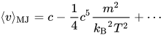
Where it follows that
c
{\displaystyle c}
References
 This article incorporates text by George Livadiotis available under the CC BY 3.0 license.
- Jüttner, F. (1911). "Das Maxwellsche Gesetz der Geschwindigkeitsverteilung in der Relativtheorie". Annalen der Physik. 339 (5): 856–882. Bibcode:1911AnP...339..856J. doi:10.1002/andp.19113390503.
- Synge, J.L (1957). The Relativistic Gas. Series in physics. North-Holland. LCCN 57003567.
- Chacon-Acosta, Guillermo; Dagdug, Leonardo; Morales-Tecotl, Hugo A. (2009). "On the Manifestly Covariant Jüttner Distribution and Equipartition Theorem". Physical Review E. 81 (2 Pt 1) 021126. arXiv:0910.1625. Bibcode:2010PhRvE..81b1126C. doi:10.1103/PhysRevE.81.021126. PMID 20365549. S2CID 39195896.
- Lazar, M.; Stockem, A.; Schlickeiser, R. (2010-12-03). "Towards a Relativistically Correct Characterization of Counterstreaming Plasmas. I. Distribution Functions". The Open Plasma Physics Journal. 3 (1).
- See first few paragraphs in for extended discussion.
- Rezzolla, Luciano; Zanotti, Olindo (2018). Relativistic hydrodynamics. Oxford: Oxford University Press. ISBN 978-0-19-852890-6.
- Dunkel, Jörn; Talkner, Peter; Hänggi, Peter (2007-05-22). "Relative entropy, Haar measures and relativistic canonical velocity distributions". New Journal of Physics. 9 (5): 144. arXiv:cond-mat/0610045. Bibcode:2007NJPh....9..144D. doi:10.1088/1367-2630/9/5/144. ISSN 1367-2630. S2CID 15896453.