In mathematics, the Prékopa–Leindler inequality is an integral inequality closely related to the reverse Young's inequality, the Brunn–Minkowski inequality and a number of other important and classical inequalities in analysis. The result is named after the Hungarian mathematicians András Prékopa and László Leindler.[1][2]
Statement of the inequality
Let 0 < λ < 1 and let f, g, h : Rn → [0, +∞) be non-negative real-valued measurable functions defined on n-dimensional Euclidean space Rn. Suppose that these functions satisfy
h
(
(
1
−
λ
)
x
+
λ
y
)
≥
f
(
x
)
1
−
λ
g
(
y
)
λ
{\displaystyle h\left((1-\lambda )x+\lambda y\right)\geq f(x)^{1-\lambda }g(y)^{\lambda }}
 | 1 |
for all x and y in Rn. Then
-
‖
h
‖
1
:=
∫
R
n
h
(
x
)
d
x
≥
(
∫
R
n
f
(
x
)
d
x
)
1
−
λ
(
∫
R
n
g
(
x
)
d
x
)
λ
=:
‖
f
‖
1
1
−
λ
‖
g
‖
1
λ
.
{\displaystyle \|h\|_{1}:=\int _{\mathbb {R} ^{n}}h(x)\,\mathrm {d} x\geq \left(\int _{\mathbb {R} ^{n}}f(x)\,\mathrm {d} x\right)^{1-\lambda }\left(\int _{\mathbb {R} ^{n}}g(x)\,\mathrm {d} x\right)^{\lambda }=:\|f\|_{1}^{1-\lambda }\|g\|_{1}^{\lambda }.}

Essential form of the inequality
Recall that the essential supremum of a measurable function f : Rn → R is defined by
-
e
s
s
s
u
p
x
∈
R
n
f
(
x
)
=
inf
{
t
∈
[
−
∞
,
+
∞
]
∣
f
(
x
)
≤
t
for almost all
x
∈
R
n
}
.
{\displaystyle \mathop {\mathrm {ess\,sup} } _{x\in \mathbb {R} ^{n}}f(x)=\inf \left\{t\in [-\infty ,+\infty ]\mid f(x)\leq t{\text{ for almost all }}x\in \mathbb {R} ^{n}\right\}.}
![{\displaystyle \mathop {\mathrm {ess\,sup} } _{x\in \mathbb {R} ^{n}}f(x)=\inf \left\{t\in [-\infty ,+\infty ]\mid f(x)\leq t{\text{ for almost all }}x\in \mathbb {R} ^{n}\right\}.}](https://wikimedia.org/api/rest_v1/media/math/render/svg/5325e3b1191b33c7ceadd098cda952a4b1701700)
This notation allows the following essential form of the Prékopa–Leindler inequality: let 0 < λ < 1 and let f, g ∈ L1(Rn; [0, +∞)) be non-negative absolutely integrable functions. Let
-
s
(
x
)
=
e
s
s
s
u
p
y
∈
R
n
f
(
x
−
y
1
−
λ
)
1
−
λ
g
(
y
λ
)
λ
.
{\displaystyle s(x)=\mathop {\mathrm {ess\,sup} } _{y\in \mathbb {R} ^{n}}f\left({\frac {x-y}{1-\lambda }}\right)^{1-\lambda }g\left({\frac {y}{\lambda }}\right)^{\lambda }.}

Then s is measurable and
-
‖
s
‖
1
≥
‖
f
‖
1
1
−
λ
‖
g
‖
1
λ
.
{\displaystyle \|s\|_{1}\geq \|f\|_{1}^{1-\lambda }\|g\|_{1}^{\lambda }.}

The essential supremum form was given by Herm Brascamp and Elliott Lieb.[3] Its use can change the left side of the inequality. For example, a function g that takes the value 1 at exactly one point will not usually yield a zero left side in the "non-essential sup" form but it will always yield a zero left side in the "essential sup" form.
Relationship to the Brunn–Minkowski inequality
It can be shown that the usual Prékopa–Leindler inequality implies the Brunn–Minkowski inequality in the following form: if 0 < λ < 1 and A and B are bounded, measurable subsets of Rn such that the Minkowski sum (1 − λ)A + λB is also measurable, then
-
μ
(
(
1
−
λ
)
A
+
λ
B
)
≥
μ
(
A
)
1
−
λ
μ
(
B
)
λ
,
{\displaystyle \mu \left((1-\lambda )A+\lambda B\right)\geq \mu (A)^{1-\lambda }\mu (B)^{\lambda },}

where μ denotes n-dimensional Lebesgue measure. Hence, the Prékopa–Leindler inequality can also be used[4] to prove the Brunn–Minkowski inequality in its more familiar form: if 0 < λ < 1 and A and B are non-empty, bounded, measurable subsets of Rn such that (1 − λ)A + λB is also measurable, then
-
μ
(
(
1
−
λ
)
A
+
λ
B
)
1
/
n
≥
(
1
−
λ
)
μ
(
A
)
1
/
n
+
λ
μ
(
B
)
1
/
n
.
{\displaystyle \mu \left((1-\lambda )A+\lambda B\right)^{1/n}\geq (1-\lambda )\mu (A)^{1/n}+\lambda \mu (B)^{1/n}.}

Applications in probability and statistics
Log-concave distributions
The Prékopa–Leindler inequality is useful in the theory of log-concave distributions, as it can be used to show that log-concavity is preserved by marginalization and independent summation of log-concave distributed random variables. Since, if
X
,
Y
{\displaystyle X,Y}


Suppose that H(x,y) is a log-concave distribution for (x,y) ∈ Rm × Rn, so that by definition we have
H
(
(
1
−
λ
)
(
x
1
,
y
1
)
+
λ
(
x
2
,
y
2
)
)
≥
H
(
x
1
,
y
1
)
1
−
λ
H
(
x
2
,
y
2
)
λ
,
{\displaystyle H\left((1-\lambda )(x_{1},y_{1})+\lambda (x_{2},y_{2})\right)\geq H(x_{1},y_{1})^{1-\lambda }H(x_{2},y_{2})^{\lambda },}
 | 2 |
and let M(y) denote the marginal distribution obtained by integrating over x:
-
M
(
y
)
=
∫
R
m
H
(
x
,
y
)
d
x
.
{\displaystyle M(y)=\int _{\mathbb {R} ^{m}}H(x,y)\,dx.}
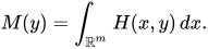
Let y1, y2 ∈ Rn and 0 < λ < 1 be given. Then equation (2) satisfies condition (1) with h(x) = H(x,(1 − λ)y1 + λy2), f(x) = H(x,y1) and g(x) = H(x,y2), so the Prékopa–Leindler inequality applies. It can be written in terms of M as
-
M
(
(
1
−
λ
)
y
1
+
λ
y
2
)
≥
M
(
y
1
)
1
−
λ
M
(
y
2
)
λ
,
{\displaystyle M((1-\lambda )y_{1}+\lambda y_{2})\geq M(y_{1})^{1-\lambda }M(y_{2})^{\lambda },}

which is the definition of log-concavity for M.
To see how this implies the preservation of log-convexity by independent sums, suppose that X and Y are independent random variables with log-concave distribution. Since the product of two log-concave functions is log-concave, the joint distribution of (X,Y) is also log-concave. Log-concavity is preserved by affine changes of coordinates, so the distribution of (X + Y, X − Y) is log-concave as well. Since the distribution of X+Y is a marginal over the joint distribution of (X + Y, X − Y), we conclude that X + Y has a log-concave distribution.
Applications to concentration of measure
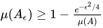
The Prékopa–Leindler inequality can be used to prove results about concentration of measure.
Theorem Let
A
⊆
R
n
{\textstyle A\subseteq \mathbb {R} ^{n}}




Proof of concentration of measure |
|---|
|
The proof of this theorem goes by way of the following lemma: Lemma In the notation of the theorem,
∫
R
n
exp
(
d
(
x
,
A
)
2
/
4
)
d
μ
≤
1
/
μ
(
A
)
{\textstyle \int _{\mathbb {R} ^{n}}\exp(d(x,A)^{2}/4)d\mu \leq 1/\mu (A)}
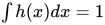
This lemma can be proven from Prékopa–Leindler by taking
h
(
x
)
=
γ
(
x
)
,
f
(
x
)
=
e
d
(
x
,
A
)
2
4
γ
(
x
)
,
g
(
x
)
=
1
A
(
x
)
γ
(
x
)
{\textstyle h(x)=\gamma (x),f(x)=e^{\frac {d(x,A)^{2}}{4}}\gamma (x),g(x)=1_{A}(x)\gamma (x)}
Since
∫
h
(
x
)
d
x
=
1
{\textstyle \int h(x)dx=1}
To conclude the concentration inequality from the lemma, note that on
R
n
∖
A
ϵ
{\textstyle \mathbb {R} ^{n}\setminus A_{\epsilon }}
|










References
- Prékopa, András (1971). "Logarithmic concave measures with application to stochastic programming" (PDF). Acta Sci. Math. 32: 301–316.
- Prékopa, András (1973). "On logarithmic concave measures and functions" (PDF). Acta Sci. Math. 34: 335–343.
- Herm Jan Brascamp; Elliott H. Lieb (1976). "On extensions of the Brunn–Minkowski and Prekopa–Leindler theorems, including inequalities for log concave functions and with an application to the diffusion equation". Journal of Functional Analysis. 22 (4): 366–389. doi:10.1016/0022-1236(76)90004-5.
- Gardner, Richard J. (2002). "The Brunn–Minkowski inequality" (PDF). Bull. Amer. Math. Soc. (N.S.). 39 (3): 355–405 (electronic). doi:10.1090/S0273-0979-02-00941-2. ISSN 0273-0979.
Further reading
- Eaton, Morris L. (1987). "Log concavity and related topics". Lectures on Topics in Probability Inequalities. Amsterdam. pp. 77–109. ISBN 90-6196-316-8.
{{cite book}}: CS1 maint: location missing publisher (link) - Wainwright, Martin J. (2019). "Concentration of Measure". High-Dimensional Statistics: A Non-Asymptotic Viewpoint. Cambridge University Press. pp. 72–76. ISBN 978-1-108-49802-9.